Learning how to use Excel doesn’t have to be difficult. Taking it one step at a time will help you move from a novice to an expert (or at least closer to that point) – at your pace. As a preview of what we are going to cover in this article, think worksheets, basic usable functions and formulas, and navigating a worksheet or workbook. Granted, we will not be covering every possible Excel function but we will cover enough that it gives you an idea of how to approach the others.
Basic Definitions
It really is helpful if we cover a few definitions. More than likely, you have heard these terms (or already know what they are). But we will cover them to be sure and be all set for the rest of the process in learning how to use Excel.
Workbooks vs. Worksheets
Excel documents are called Workbooks and when you first create an Excel document (the workbook), many (not all) Excel versions will automatically include three tabs, each with its own blank worksheet. If your version of Excel doesn’t do that, don’t worry, we will learn how to create them. The Worksheets are the actual parts where you enter the data. If it is easier to think of it visually, think of the worksheets as those tabs. You can add tabs or delete tabs by right-clicking and choosing the delete option. Those worksheets are the actual spreadsheets with which we work and they are housed in the workbook file.
The Ribbon
The Ribbon spreads across the Excel application like a row of shortcuts, but shortcuts that are represented visually (with text descriptions). This is helpful when you want to do something in short order and especially when you need help determining what you want to do. There is a different grouping of ribbon buttons depending on which section/group you choose from the top menu options (i.e. Home, Insert, Data, Review, etc.) and the visual options presented will relate to those groupings.
Excel Shortcuts
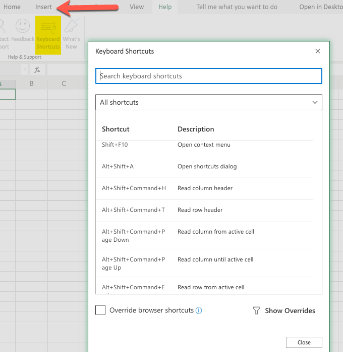
Shortcuts are helpful in navigating the Excel software quickly, so it is helpful (but not absolutely essential) to learn them. Some of them are learned by seeing the shortcuts listed in the menus of the older versions of the Excel application and then trying them out for yourself. Another way to learn Excel shortcuts is to view a list of them on the website of the Excel developers. Even if your version of Excel doesn’t display the shortcuts, most of them still work.
Formulas vs. Functions
Functions are built-in capabilities of Excel and are used in formulas. For example, if you wanted to insert a formula that calculated the sum of numbers in different cells of a spreadsheet, you could use the function SUM() to do just that. More on this function (and other functions) a bit further on in this article.
Formula Bar
The formula bar is an area that appears below the Ribbon. It is used for formulas and data. You enter the data in the cell and it will also appear in the formula bar if you have your mouse on that cell. When we reference the formula bar, we are simply indicating that we should type the formula in that spot while having the appropriate cell selected (which, again, will automatically happen if you select the cell and start typing).
Creating & Formatting a Worksheet Example
There are many things you can do with your Excel Worksheet. We will give you some example steps as we go along in this article so you can try them out for yourself.
The First Workbook
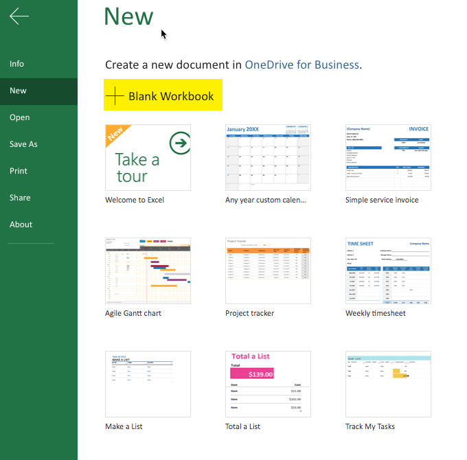
It is helpful to start with a blank Workbook. So, go ahead and select New. This may vary, depending on your version of Excel, but is generally in the File area. Note: The above image says Open at the top to illustrate that you can get to the New (left-hand side, pointed to with the green arrow) from anywhere. This is a screenshot of the newer Excel. When you click on New you are more than likely going to get some example templates. The templates themselves may vary between versions of Excel, but you should get some sort of selection. One way of learning how to use Excel is to play with those templates and see what makes them “tick”. For our article, we are starting with a blank document and playing around with data and formulas, etc. So go ahead and select the blank document option. The interface will vary, from version to version, but should be similar enough to get the idea. A little later we will also download another sample Excel sheet.
Inserting the Data
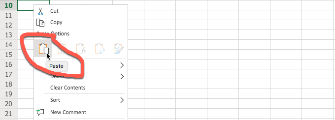
There are many different ways to get data into your spreadsheet (a.k.a. worksheet). One way is to simply type what you want where you want it. Choose the particular cell and just start typing. Another way is to copy data and then paste it into your Spreadsheet. Granted, if you are copying data that is not in a table format it can get a little interesting as to where it lands in your document. But fortunately we can always edit the document and recopy and paste elsewhere, as needed. You can try the copy/paste method now by selecting a portion of this article, copying it, and then pasting into your blank spreadsheet. After selecting the portion of the article and copying it, go to your spreadsheet and click on the desired cell where you want to start the paste and do so. The method shown above is using the right-click menu and then selecting “Paste” in the form of the icon. It is possible that you may get an error when using the Excel built-in paste method, even with the other Excel built-in methods as well. Fortunately, the error warning (above) helps to point you in the right direction to get the data you copied into the sheet. When pasting the data, Excel does a pretty good job of interpreting it. In our example, I copied the first two paragraphs of this section and Excel presented it in two rows. Since there was an actual space between the paragraphs, Excel reproduced that as well (with a blank row). If you are copying a table, Excel does an even better job of reproducing it in the sheet. Also, you can use the button in the Ribbon to paste. For visual people, this is really helpful. It is shown in the image below. Some versions of Excel (especially the older versions) allow you to import data (which works best with similar files or CSV – comma-separated values – files). Some newer versions of Excel do not have that option but you can still open the other file (the one that you want to import), use a select all and then copy and paste it into your Excel spreadsheet. When import is available, it is generally found under the File menu. In the new version(s) of Excel, you may be rerouted to more of a graphical user interface when you click on File. Simply click the arrow in the top left to return back to your worksheet.
Hyperlinking
Hyperlinking is fairly easy, especially when using the Ribbon. You will find the hyperlink button under the Insert menu in the newer Excel versions. It may also be accessed via a shortcut like command-K.
Formatting Data (Example: Numbers and Dates)
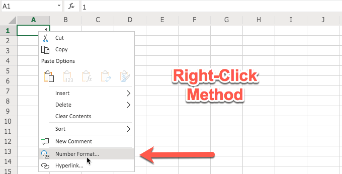
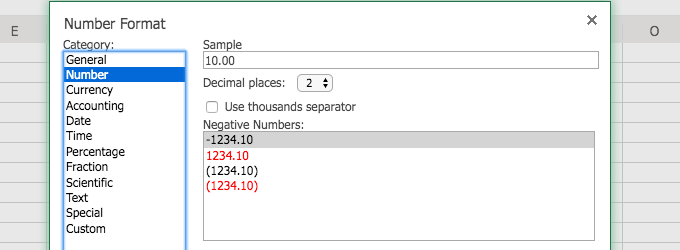
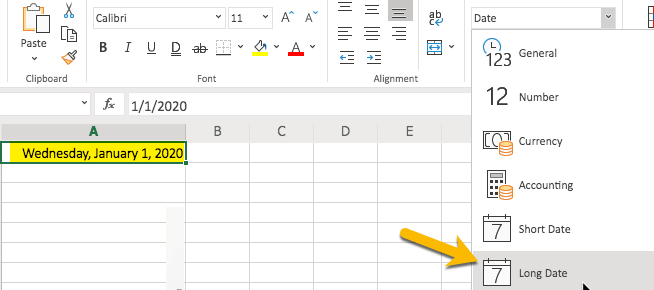
Sometimes it is helpful to format the data. This is especially true with numbers. Why? Sometimes numbers automatically fall into a general format (sort of default) which is more like a text format. But often, we want our numbers to behave as numbers. The other example would be dates, which we may want to format to ensure that all of our dates appear consistent, like 20200101 or 01/01/20 or whatever format we choose for our date format. You can access the option to format your data in a couple of different ways, shown in the below images. Once you have accessed, say, the Number format, you will have several options. These options appear when you use the right-click method. When you use the Ribbon, your options are right there in the Ribbon. It all depends on which is easier for you. If you have been using Excel for a while, the right-click method, with the resulting number format dialog box (shown below) may be easier to understand. If you are newer or more visual, the Ribbon method may make more sense (and much quicker to use). Both provide you with number formatting options. If you type anything that resembles a date, the newer versions of Excel are nice enough to reflect that in the Ribbon as shown in the below image. From the Ribbon you can select formats for your date. For example, you can choose a short date or a long date. Go ahead and try it and view your results.
Presentation Formatting (Example: Aligning Text)
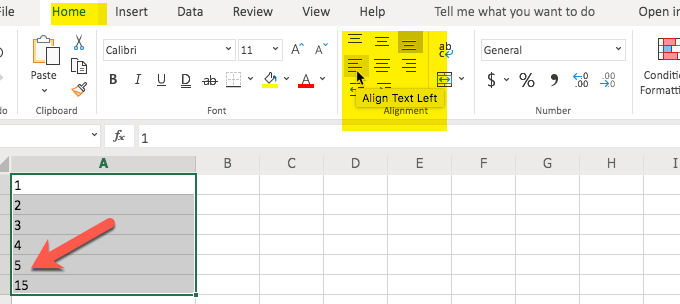
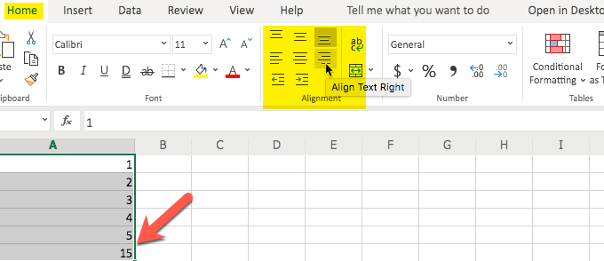
It is also helpful to understand how to align your data, whether you want it all to line up to the left or to the right (or justified, etc). This too can be accessed via the Ribbon. As you can see from the images above, the alignment of the text (i.e. right, left, etc.) is on the second row of the Ribbon option. You can also choose other alignment options (i.e. top, bottom) in the Ribbon. Also, if you notice, aligning things like numbers may not look right when aligned left (where text looks better) but does look better when aligned right. The alignment is very similar to what you would see in a word processing application.
Columns & Rows
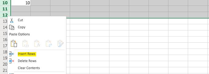
It is helpful to know how to work with, as well as adjust the width and dimensions of, columns and rows. Fortunately, once you get the hang of it, it is fairly easy to do. There are two parts to adding or deleting rows or columns. The first part is the selection process and the other is the right-click and choosing the insert or delete option. Remember the data we copied from this article and pasted into our blank Excel sheet in the above example? We probably don’t need it anymore so it is a perfect example for the process of deleting rows. Remember our first step? We need to select the rows. Go ahead and click on the row number (to the left of the top left cell) and drag downward with your mouse to the bottom row that you want to delete. In this case, we are selecting three rows. Then, the second part of our procedure is to click on Delete Rows and watch Excel delete those rows. The process for inserting a row is similar but you do not have to select more than one row. Excel will determine where you click is where you want to insert the row. To start the process, click on the row number that you want to be below the new row. This tells Excel to select the entire row for you. From the spot where you are, Excel will insert the row above that. You do so by right-clicking and choosing Insert Rows. As you can see above, we typed 10 in row 10. Then, after selecting 10 (row 10), right-clicking, and choosing Insert Rows, the number 10 went down one row. It resulted in the 10 now being in row 11. This demonstrates how the inserted row was placed above the selected row. Go ahead and try it for yourself, so you can see how the insertion process works. If you need more than one row, you can do so by selecting more than one row and this tells Excel how many you want and that quantity will be inserted above the row number selected. The following pictures show this in a visual format, including how the 10 went down three rows, the number of rows inserted. Inserting and deleting columns is basically the same except that you are selecting from the top (columns) instead of the left (rows).
Filters & Duplicates
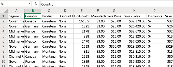
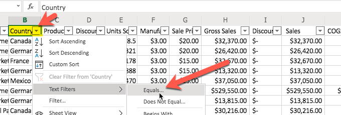
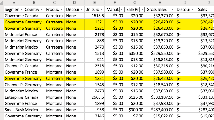
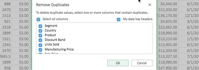
When we have a lot of data to work with it helps if we have a couple of tricks up our sleeves in order to more easily work with that data. For example, let’s say you have a bunch of financial data but you only need to look at specific data. One way to do that is to use an Excel “Filter.” First, let’s find an Excel Worksheet that presents a lot of data so we have something to test this on (without having to type all of the data ourselves). You can download just such a sample from Microsoft. Keep in mind that that is the direct link to the download so the Excel example file should start downloading right away when you click on that link. Now that we have the document, let’s look at the volume of data. Quite a bit, isn’t it? Note: the image above will look a bit different from what you have in your sample file and that is normal. Let’s say you only wanted to see data from Germany. Use the “Filter” option in the Ribbon (under “Home”). It is combined with the “Sort” option towards the right (in the newer Excel versions). Now, tell Excel what options you want. In this case, we are looking for data on Germany as the selected country. You will notice that when you select the filter option, little pull-down arrows appear in the columns. When an arrow is selected, you have several options, including the “Text Filters” option that we will be using. You have an option to sort ascending or descending. It makes sense why Excel combines these in the Ribbon since all of these options appear in the pull-down list. We will be selecting the “Equals…” under the “Text Filters.” After we select what we want to do (in this case Filter), let’s provide the information/criteria. We would like to see all the data from Germany so that is what we type in the box. Then, click “OK.” You will notice that now we only see data from Germany. The data has been filtered. The other data is still there. It is just hidden from view. There will come a time when you want to discontinue the filter and see all of the data. Simply return to the pull-down and choose to clear the filter, as shown in the below image. Sometimes you will have data sets that include duplicate data. It is much easier if you only have singular data. For example, why would you want the exact same financial data record twice (or more) in your Excel Worksheet? Below is an example of a data set that has some data that is repeated (shown highlighted in yellow). To remove duplicates (or more, as in this case), start by clicking on one of the rows that represents the duplicate data (that contains the data that is repeated). This is shown in the below image. Now, visit the “Data” tab or section and from there, you can see a button on the Ribbon that says “Remove Duplicates.” Click that. The first portion of this process presents you with a dialog box similar to what you see in the below image. Don’t let this confuse you. It is simply asking you which column to look at when identifying the duplicate data. For example, if you had several rows with the same first and last name but basically gibberish in the other columns (like a copy/paste from a website for example) and you only needed unique rows for the first and last name, you would select those columns so that the gibberish that may not be duplicate does not come into consideration in removing the excess data. In this case, we left the selection as “all columns” because we had duplicated rows manually so we knew that all of the columns were exactly the same in our example. (You can do the same with the Excel example file and test it.) After you click “OK” on the above dialog box, you will see the result and in this case, three rows were identified as matching and two of them were removed. Now, the resulting data (shown below) matches the data we started with before we went through the addition and removal of duplicates. You have just learned a couple tricks. These are especially helpful when dealing with larger data sets. Go ahead and try some other buttons that you see on the Ribbon and see what they do. You can also duplicate your Excel example file if you want to retain the original form. Rename the file you downloaded and re-download another copy. Or duplicate the file on your computer. What I did was duplicate the tab with all of the financial data (after copying it into my other example file, the one we started with that was blank) and with the duplicate tab I had two versions to play with at will. You can try this by using the right-click on the tab and choosing “Duplicate.”
Conditional Formatting
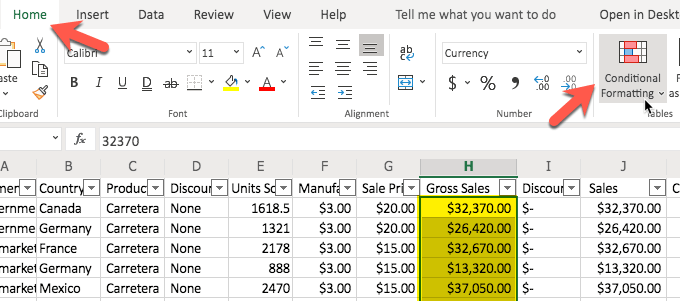
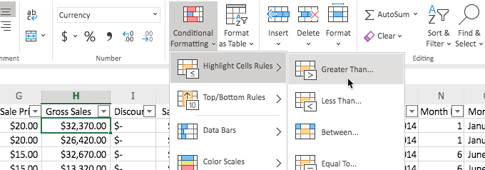
This part of the article is included in the section on creating the Workbook because of its display benefits. If it seems a little complicated or you are looking for functions and formulas, skip this section and come back to it at your leisure. Conditional Formatting is handy if you want to highlight certain data. In this example, we are going to use our Excel Example file (with all of the financial data) and look for the “Gross Sales” that are over $25,000. In order to do this, we first have to highlight the group of cells that we want evaluated. Now, keep in mind, you do not want to highlight the entire column or row. You only want to highlight just the cells that you want evaluated. Otherwise, the other cells (like headings) will also be evaluated and you would be surprised what Excel does with those headings (as an example). So, we have our desired cells highlighted and now we click on the “Home” section/group and then “Conditional Formatting.” When we click on “Conditional Formatting” in the Ribbon, we have some options. In this case we want to highlight the cells that are greater than $25,000 so that is how we make our selection, as shown in the below image. Now we will see a dialog box and we can type the value in the box. We type 25000. You don’t have to worry about commas or anything and in fact, it works better if you just type in the raw number. After we click “OK” we will see that the fields are automatically colored according to our choice (to the right) in our “Greater Than” above dialog box. In this case, “Light Red Fill with Dark Red Text). We could have chosen a different display option as well. This conditional formatting is a great way to see, at a glance, data that is essential for one project or another. In this case, we could see the “Segments” (as they are referred to in the Excel Example file) that have been able to exceed $25,000 in Gross Sales.
Working With Formulas and Functions
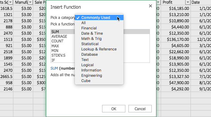
Learning how to use functions in Excel is very helpful. They are the basic guts of the formulas. If you want to see a listing of the functions to get an idea of what is available, click on the “Insert” menu/group and then at the far left, choose “Function/Functions.” Even though the purpose of this button in the Excel Ribbon is to insert an actual function (which can also be accomplished by typing in the formula bar, starting with an equals sign and then starting to type the desired function), we can also use this to see what is available. You can scroll through the functions to get a sort of idea of what you can use in your formulas. Granted, it is also very helpful to simply try them out and see what they do. You can select the group that you want to peruse by choosing a category, like “Commonly Used” for a shorter list of functions but a list that is often used (and for which some functions are covered in this article). We will be using some of these functions in the examples of the formulas we discuss in this article.
The Equals = Sign
The equals sign ( = ) is very important in Excel. It plays an essential role. This is especially true in the cases of formulas. Basically, you don’t have a formula without preceding it with an equals sign. And without the formula, it is simply the data (or text) you have entered in that cell. So just remember that before you are asking Excel to calculate or automate anything for you, that you type an equals sign ( = ) in the cell. If you include a $ sign, that tells Excel not to move the formula. Normally, the auto adjustment of formulas (using what is called relative cell references), to changes in the worksheet, is a helpful thing but sometimes you may not want it and with that $ sign, you are able to tell Excel that. You simply insert the $ in front of the letter and number of the cell reference. So a relative cell reference of D25 becomes $D$25. If this part is confusing, don’t worry about it. You can come back to it (or play with it with an Excel blank workbook).
The Awesome Ampersand » &
The ampersand ( & ) is a fun little formula “tool,” allowing you to combine cells. For example, let’s say that you have a column for first names and another column for last names and you want to create a column for the full name. You can use the & to do just that. Let’s try it in an Excel Worksheet. For this example, let’s use a blank sheet so we don’t interrupt any other project. Go ahead and type your first name in A1 and type your last name in B1. Now, to combine them, click your mouse on the C1 cell and type this formula: =A1 & “ “ & B1. Please only use the part in italics and not any of the rest of it (like not using the period). What do you see in C1? You should see your full name complete with a space between your first and last names, as would be normal in typing your full name. The & “ “ & portion of the formula is what produced that space. If you had not included “ “ you would have had your first name and last name without a space between them (go ahead and try it if you want to see the result). Another similar formula uses CONCAT but we will learn about that a little later. For now, keep in mind what the ampersand ( & ) can do for you as this little tip comes in handy in many situations.
SUM() Function
The SUM() function is very handy and it does just what it describes. It adds up the numbers you tell Excel to include and gives you the sum of their values. You can do this in a couple of different ways.
We started by typing in some numbers so we had some data to work with in the use of the function. We simply used 1, 2, 3, 4, 5 and started in A1 and typed in each cell going downward toward A5.
Now, to use the SUM() function, start by clicking in the desired cell, in this case we used A6, and typing =SUM( in the formula bar. In this example, stop when you get to the first “(.” Now, click in A1 (the top-most cell) and drag your mouse to A5 (or the bottom-most cell you want to include) and then return to the formula bar and type the closing “).” Do not include the periods or quotation marks and just the parentheses.
The other way to use this function is to manually type the information in the formula bar. This is especially helpful if you have quite a few numbers and scrolling to grab them is a bit difficult. Start this method the same way that you did for the example above, with “=SUM(.”
Then, type the top-most cell’s cell reference. In this case, that would be A1. Include a colon ( : ) and then type the bottom-most cell’s cell reference. In this case, that would be A5.
AVERAGE() Function
What if you wanted to figure out what the average of a group of numbers was? You can easily do that with the AVERAGE() function. You will notice, in the steps below, that it is basically the same as the SUM() function above but with a different function. With that in mind, we start by selecting the cell we want to use for the result (in this case A6) and then start typing with an equals sign ( = ) and the word AVERAGE. You will notice that as you begin typing it you are offered suggestions and can click on AVERAGE instead of typing the full word, if you like. Ensure that you have an opening parenthesis in your formula before we add our cell range. Otherwise, you will receive an error. Now that we have “=AVERAGE(“ typed in our A6 cell (or whichever cell you are using for the result) we can select the cell range that we want to use. In this case we are using A1 through A5. Keep in mind that you can also type it in manually rather than using the mouse to select the range. If you have a large data set typing in the range is probably easier than the scrolling that would be required to select it. But, of course, it is up to you. To complete the process simply type in the closing parenthesis “)” and you will receive the average of the five numbers. As you can see, this process is very similar to the SUM() process and other functions. Once you get the hang of one function, the others will be easier.
COUNTIF() Function
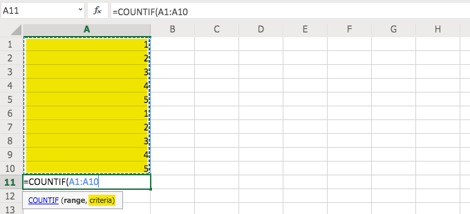
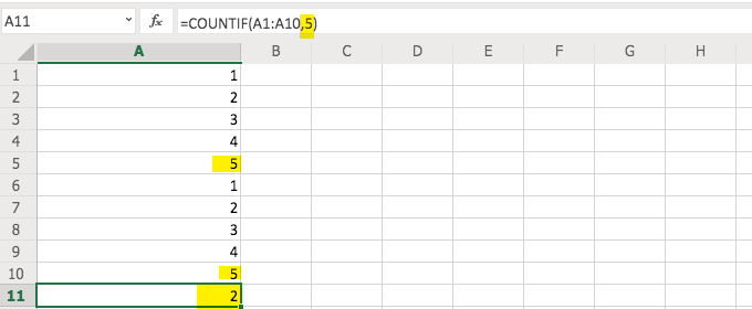
Let’s say we wanted to count how many times a certain number shows up in a data set. First, let’s prepare our file for this function so that we have something to count. Remove any formula that you may have in A6. Now, either copy A1 through A5 and paste starting in A6 or simply type the same numbers in the cells going downward starting with A6 and the value of 1 and then A7 with 2, etc. Now, in A11 let’s start our function/formula. In this case, we are going to type “=COUNTIF(.” Then, we will select cells A1 through A10. Be sure that you type or select “COUNTIF” and not one of the other COUNT-like functions or we will not get the same result. Before we do like we have with our other functions, and type the closing parenthesis “)” we need to answer the question of criteria and type that, after a comma “,” and before the parenthesis “).” What is defined by the “criteria?” That is where we tell Excel what we want it to count (in this case). We typed a comma and then a “5” and then the closing parenthesis to obtain the count of the number of fives (5) that appear in the list of numbers. That result would be two (2) as there are two occurrences.
CONCAT or CONCANTENATE() Function
Similar to our example using just the ampersand ( & ) in our formula, you can combine cells using the CONCAT() function. Go ahead and try it, using our same example. Type your first name in A1 and your last name in B1. Then, in C1 type CONCAT(A1, “ “ , B1). You will see that you get the same result as we did with the ampersand (&). Many people use the ampersand because it is easier and less cumbersome but now you see that you also have another option. Note: This function may be CONCANTENATE in your version of Excel. Microsoft shortened the function name to just CONCAT and that tends to be easier to type (and remember) in the later versions of the software. Fortunately, if you start typing CONCA in your formula bar (after the equals sign), you will see which version your version of Excel uses and can select it by clicking on it with the mouse.. Remember that when you start to type it, to allow your version of Excel to reveal the correct function, to only type “CONCA” (or shorter) and not “CONCAN” (as the start for CONCANTENATE) or you may not see Excel’s suggestion since that is where the two functions start to differ. Don’t be surprised if you prefer to use the merge method with the ampersand (&) instead of CONCAT(). That is normal.
If/Then Formulas
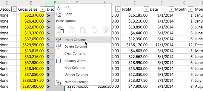
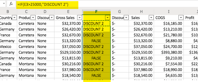
Let’s say we want to use an If/Then Formula to identify Discount (sort of a second discount) amount in a new column in our Example Excel file. In that case, first we start by adding a column and we are adding it after Column F and before Column G (again, in our downloaded example file). Now, we type in the formula. In this case, we type it in F2 and it is “=IF(E2>25000, “DISCOUNT 2”). This fulfills what the formula is looking for with a test (E2 greater than 25k) and then a result if the number in E2 passes that test (“DISCOUNT 2”). Now, copy F2 and paste in the cells that follow it in the F column. The formula will automatically adjust for each cell (relative cell referencing), with a reference to the appropriate cell. Remember that if you do not want it to automatically adjust, you can precede the cell alpha with a $ sign as well as the number, like A1 is $A$1. You can see, in the image above, that “DISCOUNT 2” appears in all of the cells in the F2 column. This is because the formula tells it to look at the E2 cell (represented by $E$2) and no relative cells. So, when the formula is copied to the next cell (i.e. F3) it is still looking at the E2 cell because of the dollar signs. So, all of the cells give the same result because they have the same formula referencing the same cell. Also, if you want a value to show up instead of the word, “FALSE,” simply add a comma and then the word or number that you want to appear (text should be in quotes) at the end of the formula, before the ending parenthesis.
Managing Your Excel Projects
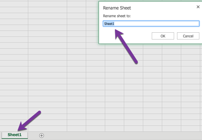
Fortunately, with the way that Excel documents are designed, you can do quite a bit with your Excel Workbooks. The ability to have different worksheets (tabs) in your document allows you to have related content all in one file. Also, if you feel that you are creating something that may have formulas that work better (or worse) you can copy (right-click option) your Worksheets (tabs) to have various versions of your Worksheet. You can rename your tabs and use date codes to let you know which versions are the newest (or oldest). This is just one example of how you can use those tabs to your advantage in managing your Excel projects. Here is an example of renaming your tabs in one of the later versions of Excel. You start by clicking on the tab and you get a result similar to the image here: If you do not receive that response, that is ok. You may have an earlier version of Excel but it is somewhat intuitive in the way that it allows you to rename the tabs. You can right-click on the tab and get an option to “rename” in the earlier versions of Excel, as well, and sometimes simply type right in the tab. Excel provides you with so many opportunities in your journey in learning how to use Excel. Now it is time to go out and use it! Have fun.


