The ability to sum data with this function isn’t limited to just two values. You can sum an entire range. And the condition you provide the function for it to sum or not can depend on multiple cells in your spreadsheet too.
How the SUMIF Function Works in Google Sheets
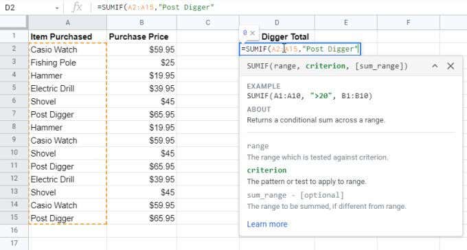
SUMIF is a simple spreadsheet function, but it’s flexible enough so that you can do some creative calculations with it. You need to frame the function as follows: SUMIF(range, criterion, [sum_range]) The parameters for this function are as follows:
Range: The range of cells you want to use to evaluate whether or not to add up the values.Criterion: The condition of the cells you want to evaluate.Sum_range: This parameter is optional, and includes the cells that you want to sum. If you don’t include this parameter, the function will simply sum up the range itself.
The function appears simple, but the fact that you can sum or compare ranges of multiple cells allows for far more flexibility than you may realize.
A SUMIF Example with Text
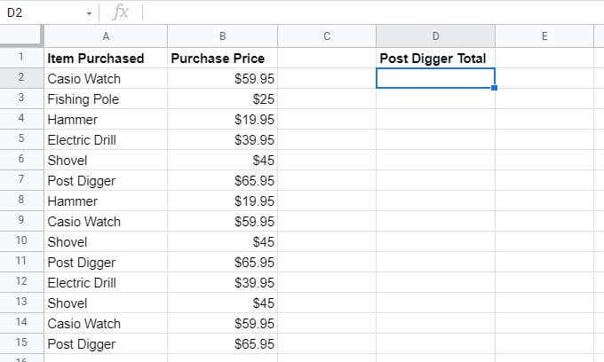
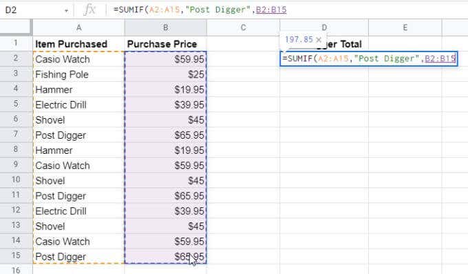
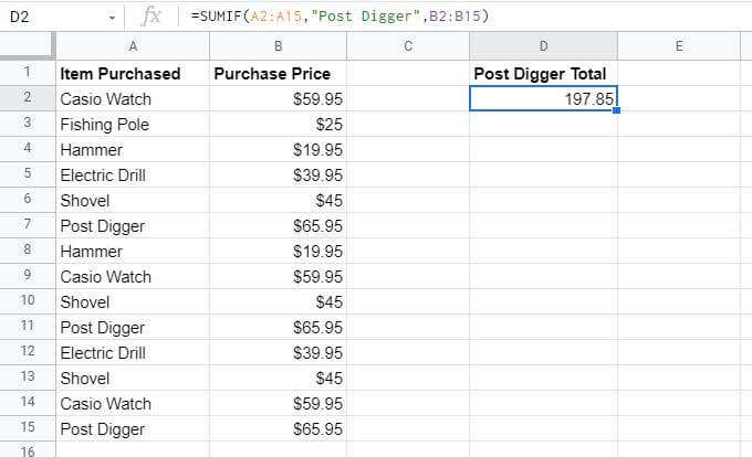
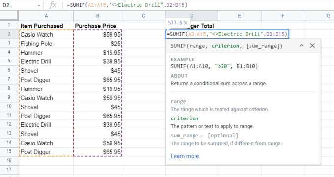
If you’re ready to get started with the SUMIF function, the best way is to use two columns in your spreadsheet. One column will be for your comparison, and the other will be the values you want to add. The example sheet above is that of a store owner who’s tracking purchases through a period. The store owner wants to create additional columns that sum up the purchase prices in column B for specific values in column A. In this case, the range for comparison would be A2:A15. The criterion would be the search phrase for the item to add up. So, in this case, to add up all of the post digger purchases, the criterion would be the text “Post Digger”. The sum range would be the range of cells with the values to be summed up. Here, this is B2:B15. When you press enter, you’ll see the specific values from the sum_range column added up, but only with the data from the cells where column A matches the criterion you specified. This is a simple way to use the SUMIF function; as a way to pluck values out of a second column based on items listed in the first. Note: You don’t have to type the criterion into the formula inside double-quotes. Instead, you could type that value into a cell in the sheet and enter that cell into the formula.
Using SUMIF Operators with Text
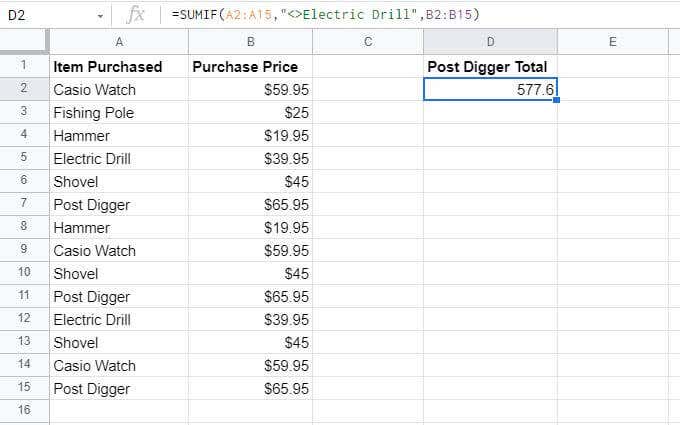
While the example above looks for perfect matches, you can also use operators to specify parts of the text you want to match. If you modify the search criteria, you can sum up values for cells that may not match perfectly but provide you with the answer you’re looking for. Using the example above, if you want to add up purchases of all items except the electric drill, you will enter the formula the <> operator. =SUMIF(A2:A15,”<>Electric Drill”,B2:B15) The <> operator tells the SUMIF function to ignore “Electric Drill” but add up all other items in the B2:B15 range. As you can see from the result below, the SUMIF function works as it should. You can also use the following operators when using the SUMIF function with text:
?: Search for words with any character where you’ve placed the ?. For example, “S?ovel” will sum any item starting with “S” and ending with “ovel” with any letter in between.*: Search for words that start or end with anything. For example, “*Watch” will add all items that are any kind of watch, regardless of brand.
Note: If you actually want the SUMIF function to search for a character like “?” or “*” in the text (and not use them as special characters), then preface those with the tilde character. For example, “~?” will include the “?” character in the search text. Keep in mind that the SUMIF function is not case-sensitive. So, it doesn’t differentiate between capital or lower-case letters when you’re using text as the search criteria. This is useful because if the same word is entered with capital letters or without, the SUMIF function will still recognize those as a match and will properly sum up the values in the value column.
Using SUMIF Operators with Numbers
Of course, the SUMIF function in Google Sheets isn’t only useful for finding text in columns with associated values to sum up. You can also sum ranges of numbers that meet certain conditions. To check a range of numbers for a condition, you can use a set of comparison operators.
: Greater than<: Less than>=: Greater than or equal to<=: Less than or equal to
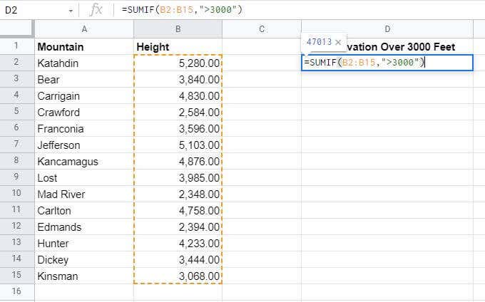
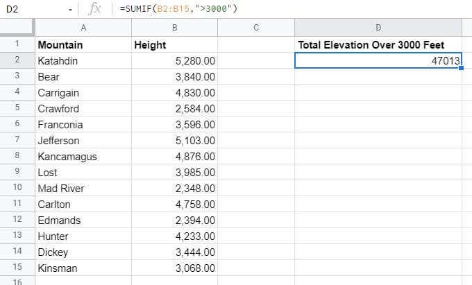
For example, if you have a list of numbers and you’d like to add those over 3000, you would use the following SUMIF command. =SUMIF(B2:B15, “>3000”) Note that just like with text criteria, you don’t need to type the number “3000” into the formula directly. You could place this number into a cell and use that cell reference instead of “3000” in the formula. Like this: =SUMIF(B2:B15, “>”&C2) One last note before we look at an example. You can also sum up all values in a range that are equal to a specific number, just by not using any comparison operators at all.
SUMIF Example with Numbers
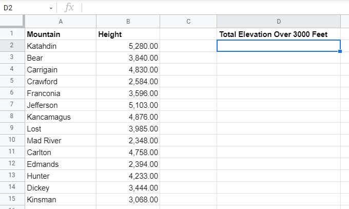
Let’s look at how you can use the SUMIF function in Google Sheets by using a comparison operator with numbers. In this example, imagine you’re a hiker tracking all the mountains that you’ve been hiking. In cell D2, you want to add up the total altitude of all of the mountains over 3000 feet that you’ve hiked. To do this, you’ll need to use the formula mentioned in the section above. Press Enter after typing the formula, and you’ll see the results in this cell. As you can see, the SUMIF function in Google Sheets summed up all altitude heights from column B for any mountain higher than 3000 feet. The SUMIF formula ignored all values under that altitude. Use the other conditional operators listed in the last section to perform the same calculation for numbers less than, greater than or equal to, less than or equal to, or equal to.
Using SUMIF Operators with Dates
You can also use the SUMIF function with dates. Again, the same comparison operators listed above apply, so you don’t have to worry about learning new ones. However, for the function to work, dates need to be formatted correctly in Google Sheets first. You can manually type the date into the function or type it into a cell and reference it into the formula. The format for this is as follows: =SUMIF(B2:B15, “>10/4/2019”, C2:C15) How this works: If you have a cell where the date isn’t formatted this way, you can use the DATE function to reformat the date properly. For example, if you have three cells (D2, D3, and D4) that hold the year, month, and day, you can use the following formula. For example: =SUMIF(B2:B15, “>”&DATE(D2, D3, D4), C2:C15) If you have a spreadsheet that contains the latest purchases at the top of the sheet, you can simply use the TODAY function to only sum up today’s purchases and ignore the rest. =SUMIF(B2:B15, TODAY())
SUMIF in Google Sheets is Simple But Versatile
As you can see, the SUMIF formula in Google Sheets doesn’t take a long time to learn. But the various ways you can use it make it so versatile. If you use many spreadsheets where you need to sum up values based on the conditions of text or numbers from other cells, you should familiarize yourself with the SUMIF function.

